Plotting basics

Matteo Ceccarello

The workflow

Building plots incrementally

We will use data from the gapminder package in these examples

# in the console
install.packages(c("tidyverse", "gapminder"))

# In your notebook
library(tidyverse)
library(gapminder)

1p <- ggplot(data = gapminder,
2            mapping = aes(x = gdpPercap,
                          y = lifeExp))
3p

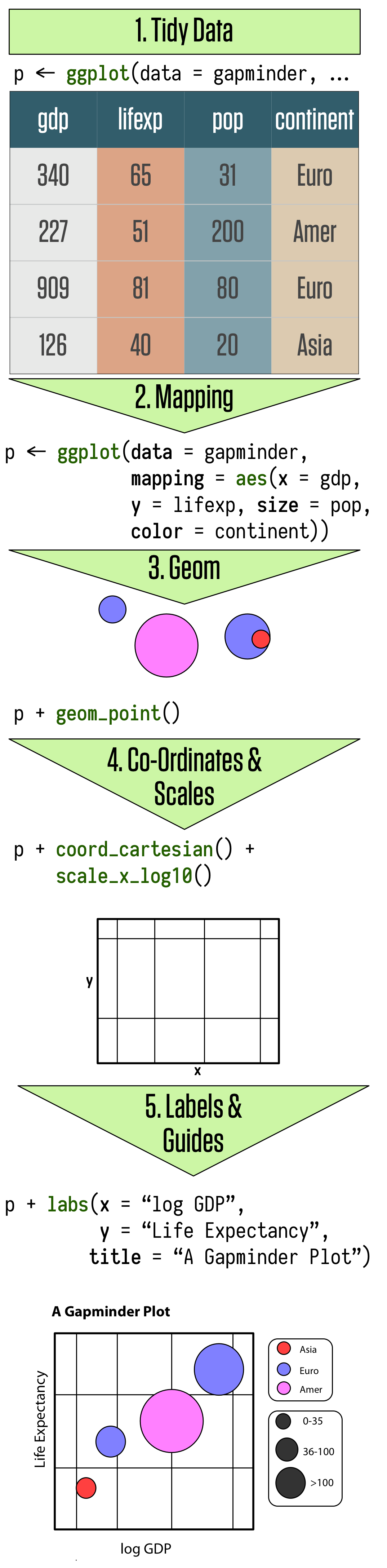
1: specify which data to use
2: say which variables to show
3: render the plot

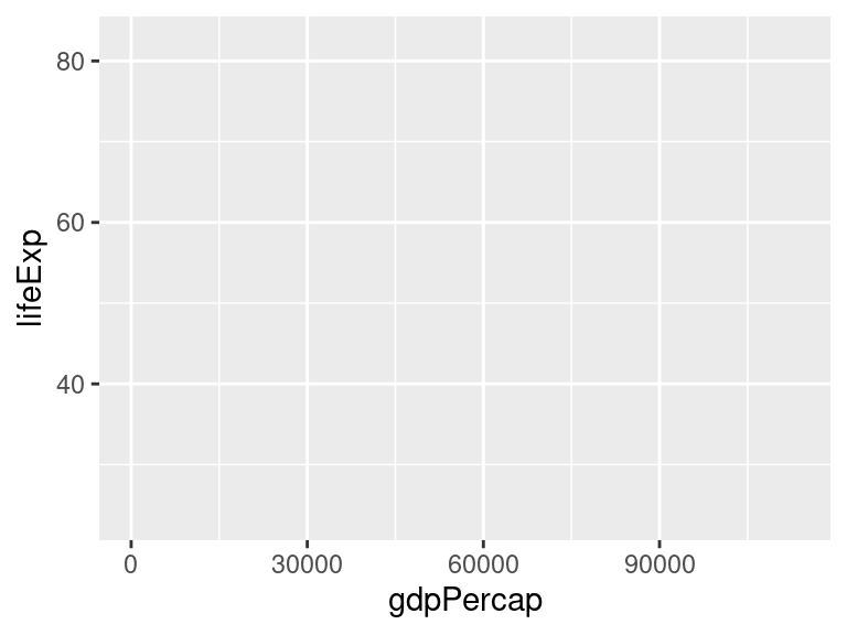
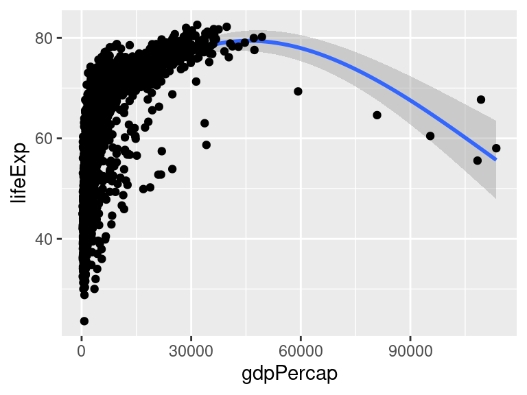
Note that the range of the axes is taken from the data

gapminder %>%
  select(gdpPercap, lifeExp) %>%
  summarise(
    minGdp = min(gdpPercap),
    maxGdp = max(gdpPercap),
    minLifeExp = min(lifeExp),
    maxLifeExp = max(lifeExp),
  )

# A tibble: 1 x 4
  minGdp  maxGdp minLifeExp maxLifeExp
   <dbl>   <dbl>      <dbl>      <dbl>
1   241. 113523.       23.6       82.6

1p +
2  geom_point()

1: “Add” something to the previously created plot. If you want to break lines, the + should be at the end, not at the beginning
2: Points are a geometric object

p +
1  geom_smooth()

1: Here we add a regression line

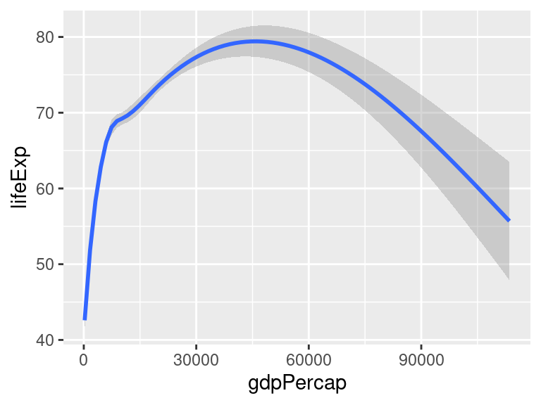
Note that points are no longer displayed: adding elements to a plot creates a new plot, leaving the input untouched.

p +
1  geom_point() +
2  geom_smooth()

1: Add points
2: Add a line

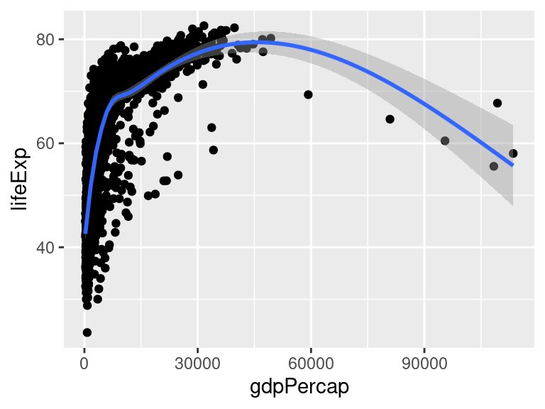
Elements can be stacked on top of each other.

What happens if we change the order?

p +
1  geom_smooth() +
2  geom_point()

1: Add a line
2: Add points

Playing with scales

p + geom_point() + 
    geom_smooth() + 
1    scale_x_log10()

1: This makes the x scale logarithmic

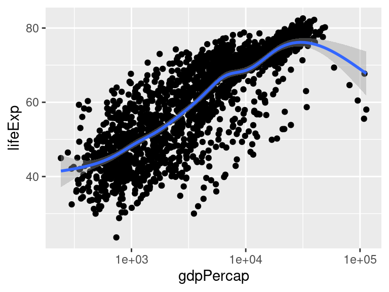
Scale transformations are applied before fitting the model line

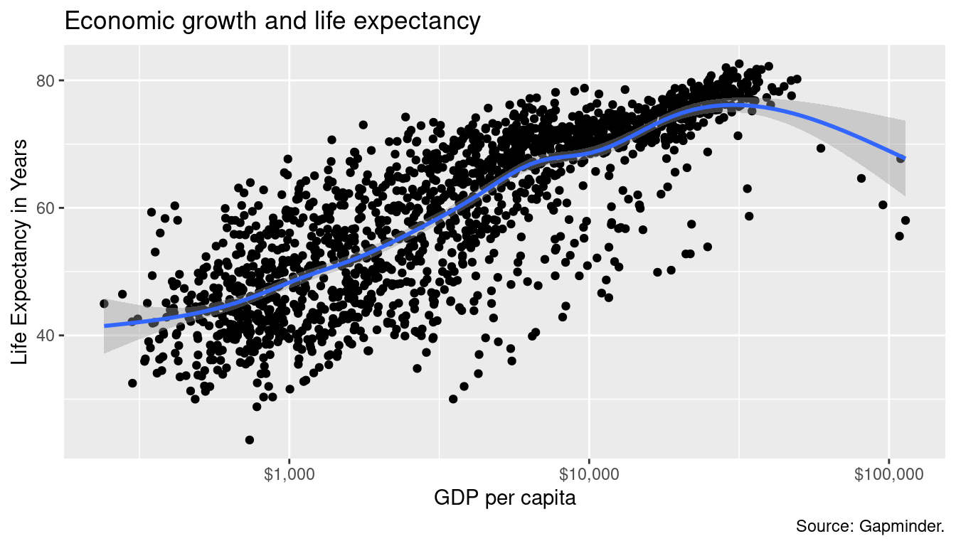
p + geom_point() + 
    geom_smooth() + 
    scale_x_log10(
1        labels = scales::dollar
    )

1: relabel the x ticks as dollars

All layers are functions, and as such they accept (optional) arguments to customize their behavior

A complete plot?

p <- ggplot(data = gapminder, 
            mapping = aes(x = gdpPercap, 
                          y = lifeExp))
p + geom_point() + 
    geom_smooth() + 
    scale_x_log10(labels = scales::dollar) +
    labs(
      x = "GDP per capita",
      y = "Life Expectancy in Years",
      title = "Economic growth and life expectancy",
      caption = "Source: Gapminder."
    )

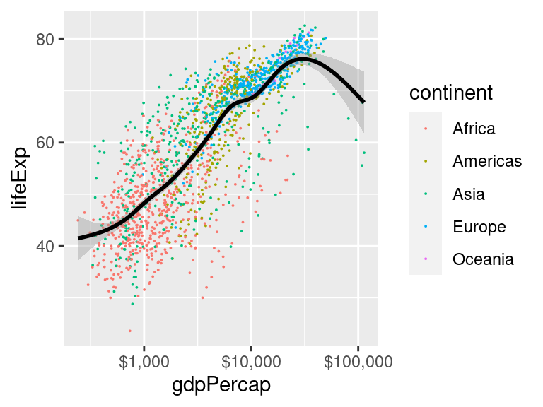
A complete plot?

What about colors?

p <- ggplot(data = gapminder, 
            mapping = aes(
              x = gdpPercap, 
              y = lifeExp, 
1              color=continent
            ))
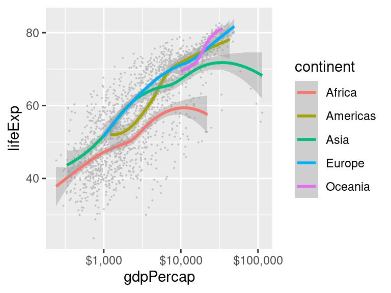
p + geom_point() + 
    geom_smooth(method = "gam") + 
    scale_x_log10(labels = scales::dollar)

1: We simply map another data variable to an aesthetic variable

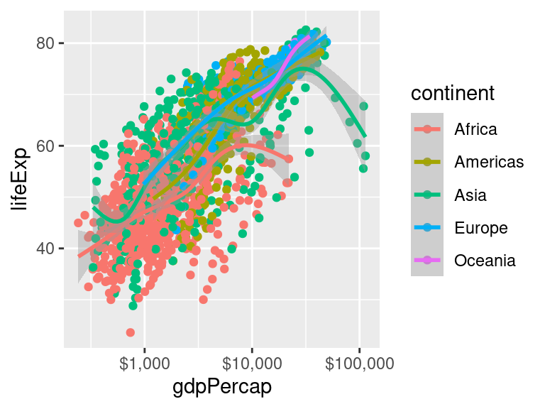
This is quite a mess! How can we address it?

Changing aesthetics for single layers

p <- ggplot(data = gapminder, 
            mapping = aes(
              x = gdpPercap, 
              y = lifeExp, 
              color=continent
            ))
p + geom_point(
    size = .01 
  ) + 
  geom_smooth() + 
  scale_x_log10(labels = scales::dollar)

Here we are fixing an aesthetic attribute to a specific value, for a single layer

Notice that, differently from before, we are not mapping a data variable to an aesthetic variable.

Changing aesthetics for single layers

p <- ggplot(data = gapminder, 
            mapping = aes(
              x = gdpPercap, 
              y = lifeExp, 
1              color=continent
            ))
p + geom_point(
    size  = .01,
2    color = "gray"
  ) + 
  geom_smooth() + 
  scale_x_log10(labels = scales::dollar)

1: Sets the default mapping for the entire plot
2: Override the mapping on a specific layer

What if?

p <- ggplot(data = gapminder, 
            mapping = aes(
              x = gdpPercap, 
              y = lifeExp, 
              color=continent
            ))
p + geom_point(
    mapping = aes(
      color = "gray"
    ),
    size  = .01
  ) + 
  geom_smooth() + 
  scale_x_log10(labels = scales::dollar)

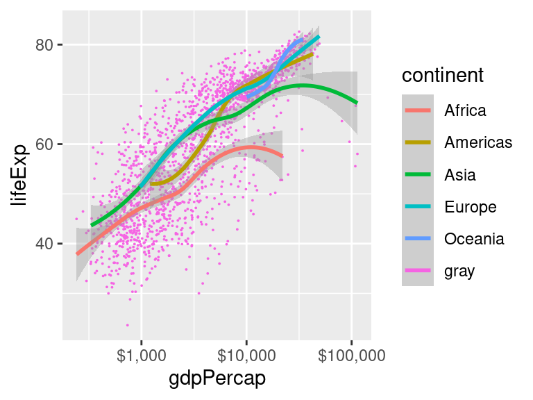
A new column consisting of all "gray" is added to the input data frame
This column is mapped to color
A color is picked from the color scale and associated to the "gray" string

Different mappings for different layers

p <- ggplot(data = gapminder, 
1            mapping = aes(
              x = gdpPercap, 
              y = lifeExp
            ))
p + geom_point(
    mapping = aes(
2      color = continent
    ),
    size  = .01
  ) + 
  geom_smooth(
3    color = "black"
  ) + 
  scale_x_log10(labels = scales::dollar)

1: No mention of continent here
2: Color points by continent
3: The smoothing layer does not know about continent, hence we get a single global smoothing line

Combining with pipelines

gapminder |>
  filter(year = 2007) |>
  ggplot(data = gapminder, 
         mapping = aes(
          x = gdpPercap, 
          y = lifeExp
        )) +
  geom_point(
    mapping = aes(
      color = continent
    ),
    size  = .01
  ) + 
  geom_smooth(
    color = "black"
  ) + 
  scale_x_log10(labels = scales::dollar)

Faceting

gapminder |>
  filter(year == 2007) |>
  ggplot(aes(
    x = gdpPercap, 
    y = lifeExp,
    color = continent
  )) + 
  geom_point() + 
  scale_x_log10(
    labels = scales::dollar,
    breaks = c(300,30000)
  ) +
  facet_wrap(
    vars(continent)
  )

Faceting

gapminder |>
  filter(year == 2007) |>
  ggplot(aes(
    x = gdpPercap, 
    y = lifeExp,
    color = continent
  )) + 
  geom_point() + 
  scale_x_log10(
    labels = scales::dollar,
    breaks = c(300,30000)
  ) +
  facet_wrap(
    vars(continent),
    ncol = 2
  )