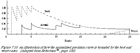
In an analogous manner normalised precision is worked out. In Figure 7.10 we once more have three curves showing (1) the best case, (2) the actual case, and (3) the worst case in terms of the precision values at different rank positions.

The calculation of the areas is a bit more messy but simple to do (see Salton[23], page 298). The area between the actual and best case is now given by:

The log function appears as a result of approximating [[Sigma]] 1/r by its continuous analogue [[integral]] 1/r dr, which is logr + constant.

The area between the worst and best case is obtained in the same way as before using the same substitution, and is:

The explicit form, with appropriate normalisation, for normalised precision is therefore:

Once again it varies between 0 (worst) and 1 (best).

A few comments about these measures are now in order. Firstly their behaviour is consistent in the sense that if one of them is 0 (or 1) then the other is 0 (or 1). In other words they both agree on the best and worst performance. Secondly, they differ in the weights assigned to arbitrary positionsof the precision-recall curve, and these weights may